Blog

The Terrain Analysis System (TAS) now available as open-source GIS project

The creator of the Terrain Analysis System (TAS) has decided to migrate his package to open source. The new version of the software, now called “Whitebox Geospatial Analysis Tools” is available for download from the department homepages.

Prof. John Lindsay is currently looking for potential graduate students (Masters) to join his research programme at the University of Guelph. Interested individuals are encouraged to contact him.

Geomorphometry 2009 logistics

Map of events

The lecture theatre during Geomorphometry 2009 is Y35F32 where Y stands for Irchel campus, 35 is the building number, F is the floor and 32 is the room number.**
Download the campus map as PDF.**

Other useful links:

[ZVV] (Zurich public transport association): Timetable, information about tickets and fares, leisure and tourist information; [SBB] (Swiss Federal Railways): Timetable, information about tickets and fares. Both the ZVV and the SBB timetables combine information about the schedules of trains, trams, busses, ships.; [Website of Zurich Tourism]: Accomodation, tours and excursions, restaurants, events etc. [Zurich Airport]: Flight, transfer and general travel information; [Zurich webcams]; [Switzerland Tourism]; [MeteoSwiss]; [Webmaps]; [Webmap of Zurich Tourism]

Number of rooms Category Name Address  
Street Postcode Place      
budget City Backpackers Niederdorfstrasse 5 8001 Zurich
budget Etap Hotel Zurich City West Technoparkstrasse 2 8005 Zurich
- budget EasyHotel Zwinglistrasse 14 8004 Zurich
155 budget Hotel Ibis Zurich City West Schiffbaustrasse 11 8005 Zurich
178 budget Hotel Ibis Zurich Messe Airport Heidi Abel-Weg 5 8050 Zurich
budget Hotel Krone Limmatquai Limmatquai 88 8001 Zurich
budget Hotel Martahaus Zaehringerstrasse 36 8001 Zurich
51 budget Hotel Sternen-Oerlikon Schaffhauserstrasse 335 8050 Zurich
budget Zurich Youth Hostel Mutschellenstrasse 114 8038 Zurich
budget ZicZac Rock Hotel Marktgasse 17 8001 Zurich
36 intermediate Best Western Hotel Zuercherhof Zaehringerstrasse 21 8021 Zurich
intermediate Best Western Hotel Montana Konradstrasse 39 8005 Zurich
54 intermediate Hotel Bristol Stampfenbachstrasse 34 8006 Zurich
70 intermediate Comfort Inn Royal Leonhardstrasse 6 8001 Zurich
40 intermediate Hotel Coronado Schaffhauserstrasse 137 8057 Zurich
78 intermediate Hotel Leoneck (Crazy Cow) Leonhardstrasse 1 8001 Zurich
intermediate Hotel Limmathof Limmatquai 142 8001 Zurich
41 intermediate Hotel Rex Weinbergstrasse 92 8006 Zurich
intermediate X-TRA Limmatstrasse 118 8005 Zurich
138 luxurious Hotel Continental Stampfenbachstrasse 60 8006 Zurich
67 luxurious Leonardo Hotel Rigihof Universitaetstrasse 101 8033 Zurich
271 luxurious Zurich Marriott Neumuehlequai 42 8001 Zurich
204 luxurious Renaissance Zurich Hotel Thurgauerstrasse 101 8152 Zurich

Hotels Conorado and Sternen-Oerlikon offer special rates for university-related stays!

For all logistics issues, please feel free to contact the logistics chief: Ralph Straumann.

Attachment: Geomorphometry2009.zip

IALE2009 Symposium6 presentations online

Perhaps some of presentations could be of interest to geomorphometrists?

Lucian Drãgut, Ulrich Walz and Thomas Blaschke have organized the 6th Symposium- The third and fourth dimensions of landscapes- within the European Conference IALE2009. The contents of presentations in the symposium, as well as introduction and concluding remarks are available below:

  1. Introduction

  2. Höchstetter & Walz- 3D-metrics in landscape ecology – Methods and examples of use

  3. Laszczak & Kozak- Assessment of structural connectivity of a forested landscape in Poland using graph theory approach

  4. Victorov- Landscape metrics selection based on the mathematical models of landscape patterns

  5. Wickham & Riiters- A critique of patch-based landscape indicators for detection of temporal change in fragmentation

  6. Van Eetvelde & Käyhkö- The applicability of quantitative techniques for assessing spatio-temporal patterns of landscape changes

  7. Werbrouck, Van Eetvelde, Antrop & De Maeyer- Integrating historical maps and LiDAR elevation data for landscape reconstruction

  8. Marceau- Scale issues in Landscape Ecology research: A synthesis

  9. Scolozzi & Geneletti- A method to assess landscape functional connectivity at local scale for target species

  10. Díaz-Varela, Álvarez-Álvarez & Marey-Pérez- Influence of landscape pattern on scale divergence in categorical maps

  11. Völker & Büker- Automatic remote sensing methods for the monitoring of agricultural landscape lements in the context of IACS and cross compliance. Poster.

  12. Stupariu, Patru-Stupariu & Cuculici- Geometric techniques in quantifying landscape irregularities. Poster.

  13. Nedkov & Gikov- Modeling landscape heterogeneity in mountain areas: a case study from Rhodope Mountains, Bulgaria. Poster.

  14. Concluding remarks

Geomorphometry in R + SAGA + ILWIS + GRASS

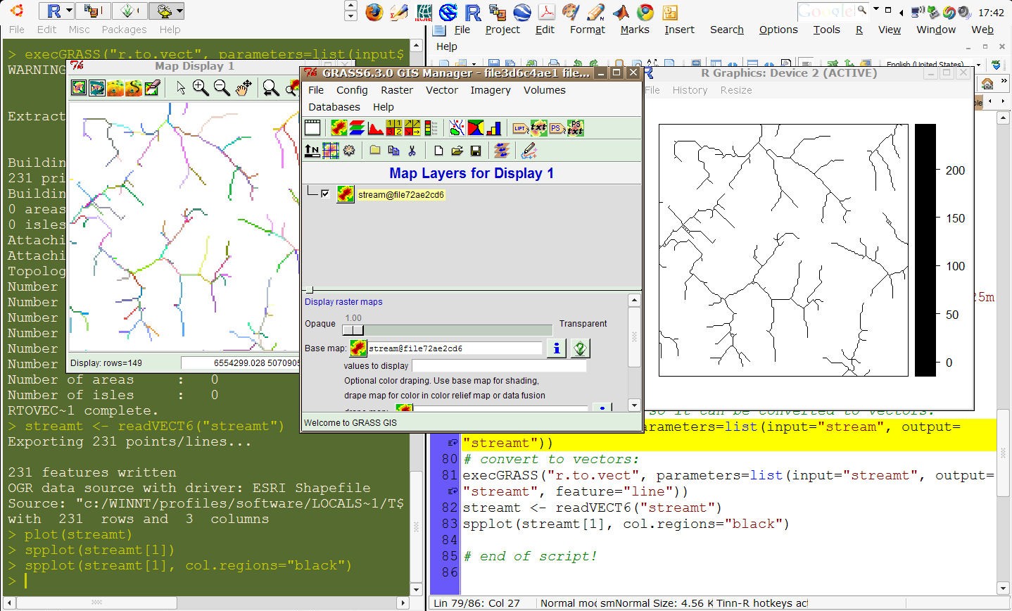
This is a sample code to process Baranja hill DEM using a combination of R, SAGA, ILWIS and Google Earth (under MS Windows machines). All four packages are available as open source or freeware (GE). You first need to obtain and install R (including the maptools, gstat, rgdal and RSAGA packages), ILWIS 3.5, SAGA GIS and GRASS GIS. After you finished installing R, SAGA, ILWIS, GRASS, copy the code down-below and start running it line by line. If you experience problems, send as a post via the R-sig-geo or ILWIS mailing list. Note: in order to use the functionality of ILWIS, SAGA, GRASS, you need to install them first. These are not internal packages in R!

Fig: Screenshots of R + SAGA/GRASS/ILWIS integration

######## R script ###############
# DEM processing and extraction of channel networks;
library(maptools)
library(rgdal)
library(RSAGA)
# ! first download and install SAGA GIS [http://www.saga-gis.org], ILWIS GIS [https://52north.org/download/Ilwis/52n-Ilwis-v3-05-02.zip] and GRASS GIS [http://grass.itc.it] to your machine!
rsaga.env(path="C:/Progra~1/saga_vc")
ILWIS <- "C:\Progra~1\N52\Ilwis35\IlwisClient.exe -C"
MGI_Z6 <- "+proj=tmerc +lat_0=0 +lon_0=18 +k=0.9999 +x_0=6500000 +y_0=0 +ellps=bessel +towgs84=550.499,164.116,475.142,5.80967,2.07902,-11.62386,0.99999445824 +units=m"
# The coordinate system is "MGI Zone 6"; see [http://spatial-analyst.net/wiki/index.php?title=MGI_/_Balkans_coordinate_systems]
setwd("C:/tmp")
# obtain the data:
download.file("http://geomorphometry.org/system/files/BaranjaHill.zip", destfile=paste(getwd(), "BaranjaHill.zip", sep="/"))
fname <- zip.file.extract(file="DEM25m.asc", zipname="BaranjaHill.zip")
file.copy(fname, "./DEM25m.asc", overwrite=TRUE)
list.files(pattern="asc")
dem25m <- readGDAL("DEM25m.asc")
proj4string(dem25m) <- CRS(MGI_Z6)
# view the data in ILWIS:
writeGDAL(dem25m[1], "dem25m.mpr", "ILWIS")
# set the right coordinate system!
download.file("http://spatial-analyst.net/CRS/gk_6.csy", destfile=paste(getwd(), "gk_6.csy", sep="/"))
shell(cmd=paste(ILWIS, "setcsy dem25m.grf gk_6.csy -force"), wait=F)
shell(cmd=paste(ILWIS, "open dem25m.mpr -noask"), wait=F)
# make a relief view in ILWIS:
shell(cmd=paste(ILWIS, "run C:\Progra~1\Ilwis3\Scripts\Hydro-DEM\dem_visualization dem25m.mpr dem25m_c.mpr"), wait=F)
# load to SAGA and derive drainage network:
rsaga.esri.to.sgrd(in.grids="dem25m.asc", out.sgrds="dem25m.sgrd", in.path=getwd())
# First, fill the spurious sinks:
rsaga.get.modules("ta_preprocessor")
rsaga.get.usage("ta_preprocessor", 2)
rsaga.geoprocessor(lib="ta_preprocessor", module=2, param=list(DEM="dem25m.sgrd", RESULT="dem25m_f.sgrd", MINSLOPE=0.05))
# Second, extract the channel network:
rsaga.get.modules("ta_channels")
rsaga.get.usage("ta_channels", 0)
rsaga.geoprocessor(lib="ta_channels", module=0, param=list(ELEVATION="dem25m.sgrd", CHNLNTWRK="channel_ntwrk.sgrd", CHNLROUTE="channel_route.sgrd", SHAPES="channels2.shp", INIT_GRID="dem25m.sgrd", DIV_CELLS=3, MINLEN=40))
channels <- readOGR("channels.shp", "channels")
spplot(channels["LENGTH"], col.regions=bpy.colors())
# derive Topographic Wetness Index:
rsaga.geoprocessor(lib="ta_hydrology", module=15, param=list(DEM="dem25m.sgrd", C="catharea.sgrd", GN="catchslope.sgrd", CS="modcatharea.sgrd", SB="TWI.sgrd", T=10))
# Export of grids to Google Earth using SAGA GIS:
rsaga.geoprocessor(lib="pj_proj4", 2, param=list(SOURCE_PROJ=paste('"', proj4string(dem25m), '"', sep=""), TARGET_PROJ=""+proj=longlat +datum=WGS84"", SOURCE="TWI.sgrd", TARGET="TWI_ll.sgrd", TARGET_TYPE=0, INTERPOLATION=0))
# export to PNG:
rsaga.geoprocessor(lib="io_grid_image", 0, param=list(GRID="TWI_ll.sgrd", FILE="TWI.png"))
# read back to R:
rsaga.sgrd.to.esri(in.sgrds="TWI_ll.sgrd", out.grids="TWI_ll.asc", prec=1, out.path=getwd())
TWI.ll <- readGDAL("TWI_ll.asc")
proj4string(TWI.ll) <- CRS("+proj=longlat +datum=WGS84")
TWI.kml <- GE_SpatialGrid(TWI.ll)
kmlOverlay(TWI.kml, kmlfile="TWI.kml", imagefile="TWI.png", name="Topographic Wetness Index")
# Optional: export to Google Earth using ILWIS:
dem25m.ll <- spTransform(dem25m[1], CRS("+proj=longlat +datum=WGS84"))
corrf <- (1+cos((dem25m.ll@bbox[2,2]+dem25m.ll@bbox[2,1])/2*pi/180))/2
geogrd.cell <- corrf*(dem25m.ll@bbox[1,2]-dem25m.ll@bbox[1,1])/dem25m@grid@cells.dim[1]
geoarc <- spsample(dem25m.ll, type="regular", cellsize=c(geogrd.cell,geogrd.cell))
gridded(geoarc) <- TRUE
gridparameters(geoarc)
gridparameters(dem25m)
# resample the map (Bilinear) to the new geographic grid:
shell(cmd=paste(ILWIS, " crgrf geoarc.grf ",geoarc@grid@cells.dim[[2]]," ",geoarc@grid@cells.dim[[1]]," -crdsys=LatlonWGS84 -lowleft=(",geoarc@grid@cellcentre.offset[[1]],",",geoarc@grid@cellcentre.offset[[2]],") -pixsize=",geoarc@grid@cellsize[[1]],sep=""), wait=F)
shell(cmd=paste(ILWIS, "dem25m_ll_c.mpr = MapResample(dem25m_c.mpr, geoarc, BiLinear)"), wait=F)
shell(cmd=paste(ILWIS, "open dem25m_ll_c.mpr -noask"))
shell(cmd=paste(ILWIS, "export tiff(dem25m_ll_c.mpr, dem25m_c.tif)"), wait=F)
# generate a KML (ground overlay):
dem25m.kml <- GE_SpatialGrid(geoarc)
kmlOverlay(dem25m.kml, "dem25m_c.kml", "dem25m_c.tif", name="Shaded relief in ILWIS")
# export of extracted channels to Google Earth:
proj4string(channels) <- CRS(MGI_Z6)
channels.ll <- spTransform(channels[3], CRS("+proj=longlat +datum=WGS84"))
writeOGR(channels.ll, "channels.kml", "channels", "KML")
# extract the drainage network in GRASS GIS:
library(spgrass6) # version => 0.6-1 (http://spatial.nhh.no/R/Devel/spgrass6_0.6-1.zip (71))
# Location of your GRASS installation:
loc <- initGRASS("C:/GRASS", home=tempdir())
loc
# Import the ArcInfo ASCII file to GRASS:
parseGRASS("r.in.gdal") # commmand description
execGRASS("r.in.gdal", flags="o", parameters=list(input="DEM25m.asc", output="DEM"))
execGRASS("g.region", parameters=list(rast="DEM"))
gmeta6()
# extract the drainage network:
execGRASS("r.watershed", flags=c("m", "overwrite"), parameters=list(elevation="DEM", stream="stream", threshold=as.integer(50)))
# thin the raster map so it can be converted to vectors:
execGRASS("r.thin", parameters=list(input="stream", output="streamt"))
# convert to vectors:
execGRASS("r.to.vect", parameters=list(input="streamt", output="streamt", feature="line"))
streamt <- readVECT6("streamt")
plot(streamt)
######## R script ###############

MORE READING:

  1. Bivand, R. 2005. Interfacing GRASS 6 and R. Status and development directions, GRASS Newsletter, 3, 11–16.
  2. Bivand, R., Pebesma, E., Rubio, V., 2008. Applied Spatial Data Analysis with R. Use R Series, p. 400. Springer, Heidelberg, pp. 378.
  3. Brenning, A. 2008. Statistical geocomputing combining R and SAGA: The example of landslide susceptibility analysis with generalized additive models. In: J. Böhner, T. Blaschke & L. Montanarella (eds.), SAGA - Seconds Out (= Hamburger Beiträge zur Physischen Geographie und Landschaftsökologie, 19), 23-32.
  4. Conrad, O. 2007. SAGA — Entwurf, Funktionsumfang und Anwendung eines Systems fur Automatisierte Geowissenschaftliche Analysen, Ph.D. thesis, University of Gottingen, Gottingen.
  5. Grohmann, C.H. 2004. Morphometric analysis in Geographic Information Systems: applications of free software GRASS and R. Computers & Geosciences, 30 (9-10):1055-1067.
  6. Hengl, T., 2009. A Practical Guide to Geostatistical Mapping. 2nd Ed, University of Amsterdam, 291 p.
  7. Neteler, M. and Mitasova, H. 2008. Open Source GIS: A GRASS GIS Approach, Springer, New York, 3rd edn.

Attachment:

SAGA_ILWIS_GRASS_0.zip

Book - Geomorphometry: Concepts, Software, Applications

A title in the Developments in Soil Science series volume 33. Read this book using the AmazonOnlineReader!

Table of content:

  • Foreword
  • **Part 1 **
  • 1. Geomorphometry: A Brief Guide
    1. Mathematical and Digital Models of the Land Surface
    1. DEM Production Methods and Sources
    1. Preparation of DEMs for Geomorphometric Analysis
    1. Geostatistical Simulation and Error Propagation in Geomorphometry
    1. Basic Land-Surface Parameters
    1. Land-Surface Parameters and Objects in Hydrology
    1. Land-Surface Parameters Specific to Topo-Climatology
    1. Landforms and Landform Elements in Geomorphometry
  • **Part 2 **
    1. Overview of Software Packages Used in Geomorphometry
    1. Geomorphometry in ESRI Packages
    1. Geomorphometry in SAGA
    1. Geomorphometry in ILWIS
    1. Geomorphometry in LandSerf
    1. Geomorphometry in MicroDEM
    1. Geomorphometry in TAS GIS
    1. Geomorphometry in GRASS GIS
    1. Geomorphometry in RiverTools
  • **Part 3 **
    1. Geomorphometry - A Key to Landscape Mapping and Modelling
    1. Soil Mapping Applications
    1. Vegetation Mapping Applications
    1. Applications in Geomorphology
    1. Modelling Mass Movements and Landslide Susceptibility
    1. Automated Predictive Mapping of Ecological Entities
    1. Geomorphometry and Spatial Hydrologic Modelling
    1. Applications in Meteorology
    1. Applications in Precision Agriculture
    1. The Future of Geomorphometry
  • Bibliography
  • Index
  • Colour Plate Section

How to cite?

The book can be cited as:

Hengl, T., Reuter, H.I. (eds) 2008. Geomorphometry: Concepts, Software, Applications. Developments in Soil Science, vol. 33, Elsevier, 772 pp.

To refer to a specific chapter, please write e.g.:

Pike, R.J., Evans, I.S., Hengl, T., 2008. Geomorphometry: a Brief Guide. In: Hengl, T. and Reuter, H.I. (Eds), Geomorphometry: Geomorphometry: Concepts, Software, Applications. Developments in Soil Science, vol. 33, Elsevier, 1-28 pp.

*Note that each specific chapter of the book has an unique DOI.

Specific chapter of the book can be obtained separately from the Elsevier’s ScienceDirect service.


How to obtain the data set?

The Baranja Hill data set used in this book can be obtained here. It comprises various data layers ranging from a TOPO DEM, SRTM DEM, original point measurements of heights, contour lines from the 1:25k and 1:5k scale topo-maps and various other thematic layers.


Attachment:

Pike_2008_Geomorphometry_ch1.pdf

Geomorphometry_bookflyer_Hengl.pdf

Latest Posts

Whitebox Workflows Next Gen released

Whitebox Workflows Next Gen, a complete rewrite of the Whitebox geospatial analysis platform, is now publicly available for Python, R, and QGIS.

Built from the ground up in pure Rust, Whitebox Next Gen provides more than 700 geospatial analysis tools for geomorphometry, terrain analysis, spatial hydrology, LiDAR processing, remote sensing, vector GIS, and spatial statistics. All three interfaces run on the same high-performance backend, allowing users to work in scripts, notebooks, statistical workflows, or a familiar desktop GIS environment.

Whitebox Next Gen is not an incremental update to the previous Whitebox architecture. It replaces the earlier monolithic system with a modular, full-stack geospatial platform. Core capabilities for raster and vector I/O, coordinate systems and reprojection, vector topology, spatial indexing, LiDAR processing, and other foundational operations are implemented directly within the Whitebox codebase rather than delegated to external C or C++ GIS libraries. This approach provides consistent cross-platform behaviour, fewer system-level dependencies, tighter control over performance and correctness, and greater flexibility for continued research and development

Highlights

  • More than 700 tools for geomorphometry, hydrology, LiDAR, remote sensing, vector analysis, spatial statistics, and general geospatial processing
  • Publicly available interfaces for Python, R, and QGIS
  • A modular, high-performance backend written entirely in Rust, including wbprojection, wbraster, wbvector, wblidar, wbspatialstats, and wbtopology open-source (MIT/Apache licensed) backend libraries
  • Most of the 80+ tools that existed within the previous extension product have been migrated to the new Whitebox open core, including the tools for advanced surface curvature analysis and DEM processing
  • Native coordinate-reference-system handling and reprojection workflows via wbprojection
  • Expanded raster support (19 formats), including GeoTIFF, Cloud-Optimized GeoTIFF (COGs), GeoPackage Raster, and JPEG2000
  • Expanded vector support (12 formats), including Shapefile, GeoPackage, FlatGeobuf, GeoParquet, GeoJSON, TopoJSON, and GML
  • Modern point-cloud support, including LAS, LAZ, COPC, E57, and PLY
  • A dedicated topology engine supporting robust vector analysis, network analysis, route-event workflows, and linear referencing
  • Local-first processing on Windows, macOS, and Linux
  • A consistent analysis platform across Python scripts and R workflows
  • A newly updated and more advanced QGIS Processing toolbox

Whitebox has particular strengths in terrain analysis, geomorphometry, spatial hydrology, and LiDAR processing. Whitebox Next Gen carries these areas forward while substantially expanding the project’s capabilities for vector analysis, remote sensing, modern spatial data formats, and reproducible geospatial workflows.

Get started

The geomorphometry community is invited to explore Whitebox Next Gen, test its tools and workflows, report issues, and contribute to the continued development of the project.

DEMIX reveals which DEMs perform best

First round of the DEMIX exercise published final report

Global digital elevation models (DEMs) have become routine operational inputs across mapping, environmental monitoring, modelling and Earth-observation workflows. Their broad coverage and global availability have made them data that many practitioners simply take for granted. But knowledge of the terrain and topography of Earth’s surface is fundamental for monitoring and understanding terrestrial ecosystems and the planet’s habitability. For that reason, the CEOS Working Group on Calibration and Validation (WGCV) maintains a subgroup dedicated to digital topography and the quality of DEMs, the ‘Terrain Mapping Sub-Group (TMSG).

DEMs are representations of elevation in the form of a georectified grid, at global scale commonly derived from space-based interferometric synthetic aperture radar (InSAR) or stereoscopic optical observations, while regionally and locally airborne Laser induced detection and ranging (LIDAR) has become the primary source. DEMs can be classified as digital surface models (DSMs) when depicting the lower surface of the atmosphere or digital terrain models (DTMs) when depicting the top of the lithosphere (the Earth’s crust).

A wide variety of DEM products exist – each having different characteristics which suit different applications. It can be challenging to understand which of the available DEM products are fit for purpose for certain applications or regions. That is the practical gap addressed by the Digital Elevation Model Intercomparison Exercise (DEMIX) undertaken by TMSG. By exposing where widely used global DEMs agree, where they differ and how those differences affect rankings, the exercise delivered evidence to users for selecting a DEM rather than defaulting to one by habit.

DEM products were compared through a ‘wine contest,’ which identified requirements of openness, reproducibility, adaptability, and statistical rigour. The characteristics, evaluations, and ranking for each DEM were collected in a GIS database with over 50,000 entries. A quantitative assessment was carried out for each global DEM based on pixel-by-pixel differences of geomorphometric parameters against finer spatial resolution (1-5 m resolution) reference DEMs.

The study incorporates an unprecedented amount of high quality reference data covering a broad range of landforms and surface types, comparing their characteristics without resampling or interpolation. Users are invited to consult the results of DEMIX in order to make informed choices when needing to use a DEM, or in some cases a combination of the most relevant DEMs for their applications.

The final rankings of the wine contest, presented below, compared the six DEMs based on land cover (forest, urban, or barren), slope (cliff, steep, gentle, or flat), differences in elevation, slope and roughness, and statistical metrics.

Led by the European Commission’s Joint Research Centre (JRC), the CEOS Working Group on Calibration and Validation (WGCV) Terrain Mapping Subgroup (TMSG) established DEMIX in partnership with the International Society for Geomorphometry. Several members of the International Society of the Geomorphometry contributed significantly and we hosted various secssions at our latest conference. The exercise was performed over a three-year period starting in 2020, with community-wide calls for participation and an assembly of experts producing a number of peer-reviewed publications, culminating with a JRC reference report published in July 2026.

The objective of DEMIX was to propose a procedure to rank the available free and open global DEMs, taking into consideration user needs while promoting the implementation of FAIR (Findable, Accessible, Interoperable and Reusable) principles. The exercise compared DEMs based on criteria for land cover and terrain slope categories, representative testing, and a statistically sound ranking approach. The report outputs tailored recommendations regarding available DEM products that are not limited to one domain, geographic area, or landscape type, with flexibility for different user needs and applications.

A major challenge in the comparison of the global DEMs were the varying formats, data, and metadata contents. The adoption of a common set of standards would enhance the quality and interoperability of global DEMs and streamline the exchange and utilisation of DEM data for both providers and users. DEMIX makes the following recommendations for data providers:

● Adopt a standardised grid layout, with complete grid definitions and encodings following ISO/OGC rules.

● Include vertical datum information as part of raster DEM files.

● Clearly indicate the product version in the file names.

● Participate in future DEMIX rounds, which serve as a neutral platform for independently evaluating products before their release.

● Provide high quality, finer resolution, accurate, and multi-temporal elevation data to be used as a reference alongside DEM products.

Global DEMs are indispensable operational geospatial datasets, but they should not be treated as error-free or interchangeable. DEMIX delivered to the global community a systematic and transparent method to help choose elevation products more intelligently and help define what better elevation measurements should look like in the future.

Further Reading:

Read more in the DEMIX Final Report, or see other DEMIX publications below - mainly by our ISG members:

  • Benchmarking Elevation Plus Land Surface Parameters Finds FathomDEM and Copernicus DEM Win as Best Global DEMs (2025) and subsequent discussion (2026a, 2026b)
  • Ranking of 10 Global One-Arc-Second DEMs Reveals Limitations in Terrain Morphology Representation 2025
  • Novel Approach for Ranking DEMs: Copernicus DEM Improves One Arc Second Open Global Topography (2024)
  • Digital Elevation Models: Terminology and Definitions (2021)
  • The Digital Elevation Model Intercomparison eXperiment DEMIX, a community-based approach at global DEM benchmarking (2021)

Coffee Talk - GeoNadir

Building the world’s largest repository of FAIR drone mapping data

Paul Mead GeoNadir

September 2nd, 2026
11:30 (UTC)

Bio: Paul Mead is Co-founder and Head of Business & Strategy at GeoNadir, a platform building the world’s largest repository of FAIR drone mapping data to support environmental decision-making. A non-technical co-founder, Paul focuses on strategy, commercial development, and building high-performing teams — a discipline shaped by 11 years in the New Zealand Army, including leading a bomb disposal team in Lebanon and service in Afghanistan and the Asia-Pacific region. Since 2013 he has built and led several small businesses and start-ups, with drones as a central technology since 2016. Alongside GeoNadir, Paul co-founded She Maps, an internationally recognised drone and geospatial STEM education organisation, and has helped raise over $7M in equity and non-equity funding across his ventures. He holds a Master of Philosophy from the University of Queensland and is a Chartered Manager.

Abstract: GeoNadir set out to build the world’s largest repository of FAIR drone mapping data, and ended up building something more powerful. Drones have democratised data capture, but the same democratised ability to generate decision-grade insights from the data is lacking. I’ll walk through how we’re closing that gap: the data infrastructure behind hosting large volumes of UAV imagery and derived products, and how we’re moving from manual analysis toward automated, repeatable geospatial analytics.